Tutorial
Introduction
This tutorial shows how to use the qmt toolbox to quickly process inertial sensor data with various algorithms.
To use qmt, simply import the qmt package:
import qmt
In a Jupyter notebook, you can use the following template to also get access to the most important packages and configure numpy printing options:
%pylab --no-import-all notebook
import qmt, os, sys, time, re, glob, itertools, math, collections
from pathlib import Path
np.set_printoptions(suppress=True)
Basic quaternion functions
Most motion tracking applications will deal with time series of quaternion data. Most functions assume that a quaternion time series of N samples will be stored in an (N, 4) numpy array.
The qmt toolbox includes many functions for the most common quaternion operations (e.g., quaternion multiplication
qmt.qmult(), inverting qmt.qinv(), calculating relative quaternions qmt.qrel()) and also for the
conversion to and from other representation (e.g., qmt.eulerAngles(), qmt.quatFromAngleAxis()) and much
more. See Python data processing functions for a list of all functions.
Here is a simple example that shows how 100 random quaternions are generated, then multiplied with a fixed 90° rotation, and then converted to Euler angles:
q1 = qmt.randomQuat(100)  # returns a (100, 4) array
q2 = qmt.quatFromAngleAxis(np.deg2rad(90), [1, 0, 0])  # returns a (4,) array
q3 = qmt.qmult(q1, q2)  # returns a (100, 4) array
angles = np.rad2deg(qmt.eulerAngles(q3, 'zxy', intrinsic=True))  # return a (100, 3) array
Debug outputs and debug plots
All data processing functions have an optional debug argument that is set to False by default. If set to
True, the function will either return an extra debug output or set the debug key in the outputs dictionary.
This debug output is a dictionary containing various signals that help understanding how the function works internally.
Furthermore, every data processing function has an optional plot argument that is set to False by default. If
set to True, a debug plot will automatically be created. You can use the function qmt.setupDebugPlots()
to configure how debug plots should behave, e.g. save them to files (or a multipage PDF!) or control the size of the
figures.
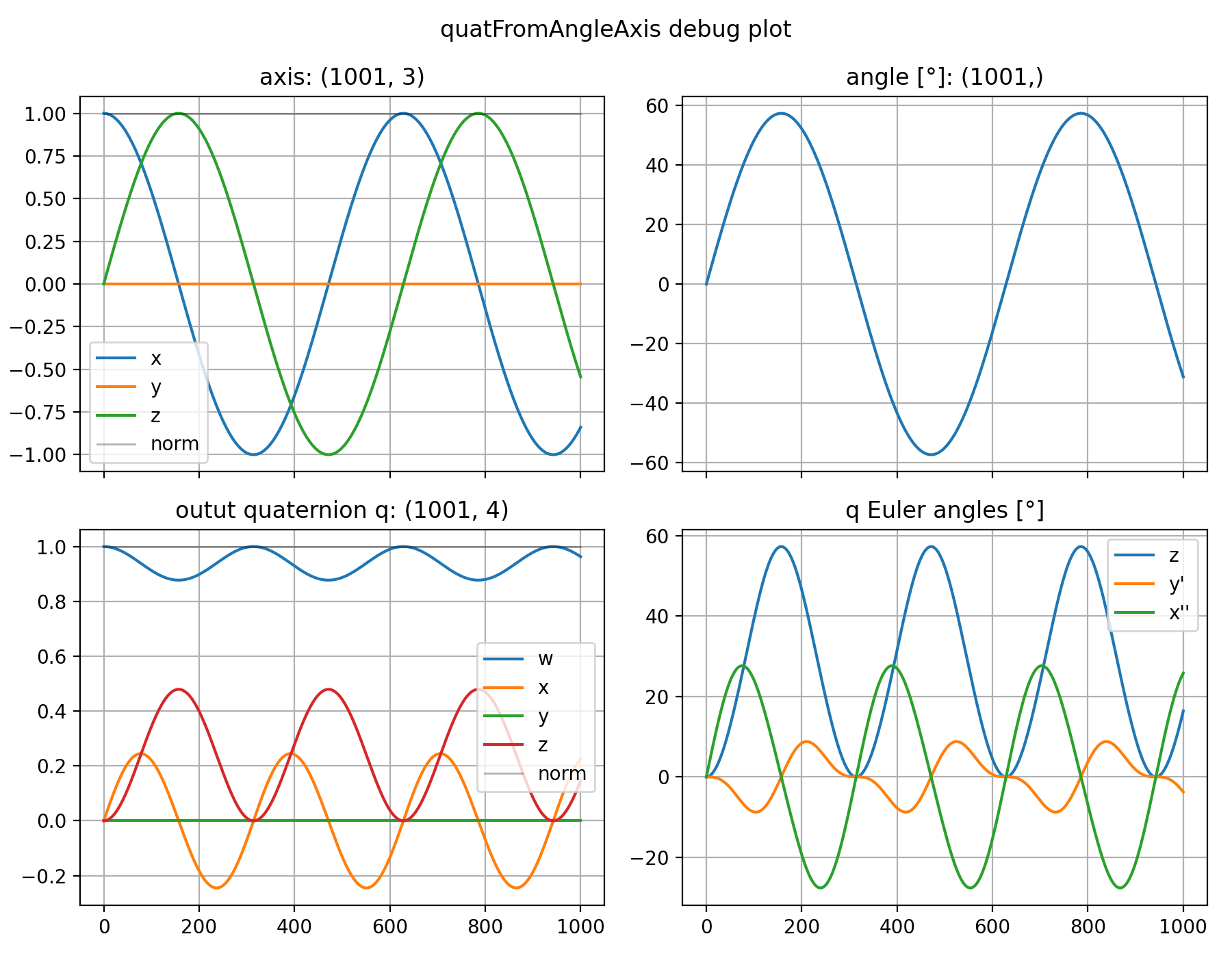
t = qmt.timeVec(T=10, Ts=0.01)
axis = np.column_stack([np.cos(t), np.zeros_like(t), np.sin(t)])
quat = qmt.quatFromAngleAxis(np.sin(t), axis, debug=True, plot=True)
(Source code, png, hires.png, pdf)

Webapps for 3D visualization
The qmt toolbox comes with a versatile system for creating web-based visualizations. The main goal of this system is to make it as easy to visualize complex kinematic chains in 3D as it is to create a line plot. For this, qmt comes with flexible apps that can display arbitrary kinematic chains as box models.
When used in Python scripts, an extra window will pop up to show the webapp. In Jupyter notebooks, the webapps can be embedded directly into the notebook.
This framework can also be used to build complex applications that read data from IMUs in realtime, process the data, create 3D visualizations and provide various controls for interaction. But for the simple case, only two lines of code are needed to open a 3D visualization:
# generate example data
t = qmt.timeVec(T=10, Ts=0.01)
axis = np.column_stack([np.cos(t), np.zeros_like(t), np.sin(t)])
quat = qmt.quatFromAngleAxis(np.sin(t), axis)
data = qmt.Struct(t=t, quat=quat)

# run webapp
webapp = qmt.Webapp('/view/imubox', data=data)
webapp.run()
There is a number of simple examples showing how to use the qmt.Webapp class for different use cases.
Please take a look at the files webapp_example_script.py and webapp_example_notebook.ipynb in the
examples/ folder.
See Webapps for a list of all available webapps and Webapp development for some information on how to create custom webapps.
For playback of stored data from .mat or .json files, there is a command-line utility called qmt-webapp. Run
qmt-webapp -h to see how to use it.
Matlab interface
Using Transplant, it is possible to call Matlab functions from Python
scripts using the qmt.matlab prefix. For example, qmt.matlab.qmult will call the Matlab function
qmt.qmult().
This will start an instance of Matlab in the background the first time a Matlab function is called. If the path does not
contain an executable with the name matlab, you will need to initialize Matlab manually before the first usage:
qmt.matlab.init(executable='/usr/local/MATLAB/R2017b/bin/matlab')
qmt.matlab provides access to functions in the +qmt Matlab package. It is possible to get access to the
full Matlab instance and execute arbitrary code in Matlab:
m = qmt.matlab.instance
print('matlab version:', m.version())
Note
Transplant will convert Python dictionaries to containers.Map by default. To pass arguments as a Matlab
struct, use a qmt.Struct.